The Influence of a Randomized SVD on the Subspace K-Means Algorithm

2018-11-06

Clustering is one of the most common forms of unsupervised machine learning algorithms, often used to discover similarity and structure in data. Clustering and dimensionality reduction techniques have huge application in a variety of fields, including bioinformatics, political science, network analysis, etc.

Among clustering algorithms, the k-means algorithm is one of the most popular partition based techniques due to its simplicity, speed, and good performance. However, it is often difficult to determine what structure k-means is finding and exploiting when clustering a dataset. Recent work has proposed an adaptation to the k-means algorithm, known as subspace k-means, that in addition to determining cluster centroids, simultaneously determines a subspace to project the clusters onto that highlights the structure of the dataset (Mautz et al., 2017). Subspace k-means makes the assumption that the features of a given dataset can be partitioned into a cluster subspace and a noise subspace. The features that belong to the cluster subspace being informative to the final clustering result, while the features belonging to the noise subspace have no bearing on the clustering result.

As the subspace k-means algorithm proceeds, it repeatedly calculates a transformation matrix, V , which rotates and reflects the original space so that the first m features in the transformed space correspond to the clustered space and the last (d−m) features correspond to the noise space, where d is the dimensionality of the dataset. In the original algorithm, the transformation matrix is determined through an eigenvalue decomposition that relies on an underlying Fortran library known as ARPACK. ARPACK uses a Krylov subspace method, either the Lanczos or Arnoldi algorithm (Van Loan et al., 1996), to compute the eigenvalue decomposition. As the dimensionality of a dataset grows, calculating the transformation matrix represents a major bottleneck of the subspace k-means algorithm in terms of computational complexity and runtime.

My colleague and I extended the original subspace k-means algorithm to incorporate recent developments in probabilistic methods for low rank matrix approximations to estimate the transformation matrix, improving runtime performance, numerical stability, and most importantly enabling this algorithm to efficiently handle large, high dimensional datasets. We also showed that our modification does not alter the mechanics of the original algorithm, providing similar subspace projections, and the same theoretical convergence guarantees.

Given how recent the subspace k-means algorithm was developed, it has received little investigation beyond the original study. We believe that our modification to the original subspace k-means algorithm provides insight into the performance of the subspace k-means algorithms when applied to high dimensional datasets, in addition to providing a practical means for applying the technique to high dimensional matrices.

Combining clustering methods with dimensionality reduction or some form of subspace projection is not a new idea. For example principle component analysis (PCA) has been combined with k-means, as has linear discriminant analysis (LDA).

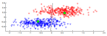
Subspace K-Means

The subspace k-means algorithm developed by Mautz et al. works similarly to vanilla k-means with the addition of a transformation matrix calculation, and a projection step. Our modifications to the algorithm involve the calculation of the transformation matrix.

The subspace k-means algorithm assumes that the relevant cluster structure of a given dataset is contained in a lower dimensional subspace. The first subspace is known as the cluster subspace, and contains all of the relevant information for partitioning the data. The second subspace is known as the noise subspace, and is orthogonal to the cluster subspace. The noise subspace does not contain any relevant information for clustering.

The crux of the algorithm relies on finding an orthonormal transformation matrix, \(V\), such that the original space is rotated and reflected so the first \(m\) features in the transformed space correspond to the cluster subspace, and the other \( (d − m) \) features correspond to the noise subspace.

To create a trade-off between the cluster and noise subspaces, subspace k-means minimizes a modified k-means objective,

\[ \mathcal{J} = \bigg[\sum_{i=1}^k \sum_{x \in C_i} ||P_C^T V^T \mathbf{x} - P_C^T V^T \mathbf{\mu}_i||^2 \bigg] + \sum_{\mathbf{x \in \mathcal{D}}} ||P_N^T V^T \mathbf{x} - P_N^T \mathbf{\mu}_{\mathcal{D}}||^2 \]

where \( P_C = \begin{bmatrix}\mathbf{I}_m & \mathbf{0}_{d-m,m} \end{bmatrix}^T \) is the cluster space projection matrix, \( P_N = \begin{bmatrix} \mathbf{0}_{m, d-m} & \mathbf{I}_{d-m} \end{bmatrix}^T \) is the noise space projection matrix, \( V \) is the transformation matrix, \( \mathcal{D} \) is the dataset, \( C_i \) is cluster \( i \), \( \mathbf{\mu}_i \) is the mean of cluster \( i \), and \( \mathbf{\mu}_\mathcal{D} \) is the dataset mean. Informative features are better represented by the first term, while uninformative features are better represented by the second term. The objective function can be rewritten as,

\[ \begin{split} \mathcal{J} & = \text{Tr} \bigg( P_C P_C^T V^T \underbrace{\bigg( \bigg[ \sum_{i=1}^k S_i \bigg] - S_\mathcal{D} \bigg)}_{=: \Sigma} V \bigg) + \underbrace{\text{Tr} (V^T S_\mathcal{D} V)}_{\text{const. w.r.t } V} \end{split} \]

where \( S_i \) is the scatter matrix for cluster \( i \), and \(S_\mathcal{D} \) is the dataset scatter matrix.

In the above cost function \( P_C P_C^T \) leaves the upper \(m \times m\) portion of the matrix unchanged and sets all other values to zero. Then, we minimize the cost function for a fixed cluster partition, fixed \(\mathbf{\mu}_i\), and fixed cluster space dimensionality \(m\), by using the eigenvectors of \(\Sigma\) as columns in the transformation matrix \(V\), such that the eigenvectors are sorted in ascending order according to the corresponding eigenvalues, such that the \(m\) eigenvectors corresponding to the \(m\) smallest eigenvalues project the data onto the cluster subspace.

We can determine the dimensionality of the cluster space $m$, by realizing that the cost function only depends on \(m\) through the projection matrix \(P_C\). Since the trace sums up the eigenvalues of the expression in the cost function, we can minimize the function by taking \(m\) to be equal to the number of negative eigenvalues in the decomposition of \(\Sigma\).

\( V \) rotates and reflects the original space so that the cluster space and noise space comprise the first \( m \) features and the last \( d-m \) features in the transformed space, respectively (where \( d \) is the dimensionality of the dataset and \( m \) is the dimensionality of the cluster space). The original algorithm's transformation matrix is determined through an eigenvalue decomposition that uses a Krylov subspace method in ARPACK with \( O(d^3) \) complexity. Consequently, as the dimensionality of a dataset grows, calculating the transformation matrix represents a major bottleneck in terms of computational complexity and runtime.

Randomized Subspace K-Means

Our modified algorithm, which we call randomized subspace k-means, modifies the calculation of the transformation matrix from the original algorithm. We can see that the objective function only depends on the upper \(m \times m\) portion of \(V\) due to the projection \(P_C P_C^T\), which sets all values besides the upper \(m \times m\) portion of the matrix to zero. Therefore, we have introduced a randomized eigenvalue decomposition to compute a rank-m approximation to \(V\).

The singular value decomposition (SVD) gives us a tool for computing a low rank approximation of a matrix \(A\). In other words, if we have a matrix \(A_r\), then our approximation will minimize some norm \(||A - A_r||\). Given \(A=U \Sigma V^T\), we can compute a low rank approximation to \(A\) by taking the \(r\) largest values of \(\Sigma\) such that we have \(\Sigma_r\) an \(r \times r\) matrix, the corresponding columns of \(U\), \(U_r\) an \(m \times r\) orthogonal matrix, and the corresponding columns of \(V\), \(V_r\) an \(n \times r\) orthogonal matrix. Then our low rank approximation is \(A_r = U_r \Sigma_r V_r^T\).

Computing the singular value decomposition for a large matrix can be an extremely time consuming operation. Randomized algorithms provide a means to speed up this operation compared to classical methods. In our work, we substitute the Lanczos and Arnoldi iteration methods used to compute the transformation matrix \(V\) in the original algorithm, with a randomized SVD method. Randomized methods are often faster, and can even be more robust than classic factorization methods.

Randomized SVD algorithms involve two major steps. Assume that we wish to find a low rank approximation for a matrix \(A\). The first step consists of using randomized techniques to compute an approximation to the range of \(A\). In other words, we want to find a \(Q\) with \(r\) orthonormal columns, such that \(A \approx Q Q^* A\), where \(Q^*\) is the conjugate transpose of \(Q\). Once we have found \(Q\), an SVD for \(A\) can be found.

We first construct \(B=Q^* A\). Since \(B\) is fairly small (due to the fact that \(Q\) has a small number of columns), the SVD of \(B\) can be efficiently computed using standard methods, so that \(B=S\Sigma V^T\), with \(S,V\) orthogonal, and \(\Sigma\) diagonal. Then as \(A\approx Q Q^* A = Q(S \Sigma V^T)\), taking \(U=QS\) shows that we have found a low rank approximation \(A \approx U \Sigma V^T\).

The randomized component of the algorithm is involved in the estimation of the matrix \(Q\). If we take a collection of random vectors \(\Omega_1, \Omega_2,...\), and examine the subspace formed by the action of \(A\) on each of these random vectors, we can estimate the range of matrix \(A\). If we form an \(n \times l\) Gaussian random matrix, \(\Omega\), compute \(Y = A \Omega\), and take the QR decomposition of \(Y\), \(QR=Y\), then \(Q\) is an \(m \times l\) matrix whose columns are an orthonormal basis for the range of \(Y\).

The randomized SVD is the most general case, and the randomized eigenvalue decomposition proceeds similarly. We want to find a \(Q\), with \(r\) orthonormal columns, such that, \(A = Q(Q^*AQ)Q^*\). We then let \(B = Q^*AQ\), and perform the eigenvalue decomposition of \(B\) with standard methods so that \(B=V \Lambda V^*\). As with the randomized SVD, since \(B\) is relatively small due to the small number of columns in \(Q\), the operation can be done quickly. Then \(A \approx Q(Q^*AQ)Q^* = Q(V \Lambda V^*)Q\). Taking \(U = QV\) shows that we have an approximation \(A \approx U \Lambda U^*\). \(Q\) is determined in the same fashion as in the randomized SVD.

With this modification, we can now express the cost function without the projection matrix as

\[ \begin{split} \mathcal{J} = \text{Tr} \bigg( V^T \underbrace{\bigg(\bigg[\sum_{i=1}^k S_i\bigg] - S_\mathcal{D} \bigg)}_{=: \Sigma} V \bigg) + \underbrace{\text{Tr} (V^T S_\mathcal{D} V)}_{\text{const. w.r.t } V}. \end{split} \]

Now that \(V\) is \(d \times m\) instead of \(d \times d\), \(V^T S_\mathcal{D} V\) in the second term is now \(m \times m\) instead of \(d \times d\); this reduces the value of \(\text{Tr}(V^T S_\mathcal{D} V)\) compared to the original objective function, but doesn't change the optimization since it is still constant for all iterations.

The cost function is decreasing in each assignment and update step, so the estimation of \(m\) does not change from the original algorithm since \(m\) will never get larger on subsequent iterations. As a result, truncating the eigenvalue decomposition using the randomized method has no effect on the estimation of the dimensionality of the cluster space. However, as we discard the \((d-m) \times (d-m)\) bottom portion of the transformation matrix we do lose the ability to view the data projected into the noise subspace.

Clustering Results

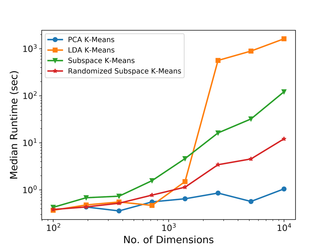
The following figures show runtime comparisons between different clustering methods as the number of data points is increased and the dimensionality of those datapoints is increased. You'll notice that compared to the original subspace k-means method, our randomized matrix decomposition modification results in an order of magnitude runtime improvement as the dimensionality of the dataset is increased.

It's also interesting to look at how the subspace projections affect the datapoints we are trying to cluster. Each of the following figures shows subsets of different datasets plotted using the first two features of the original feature space on the left and the first two features of the cluster subspace on the right.

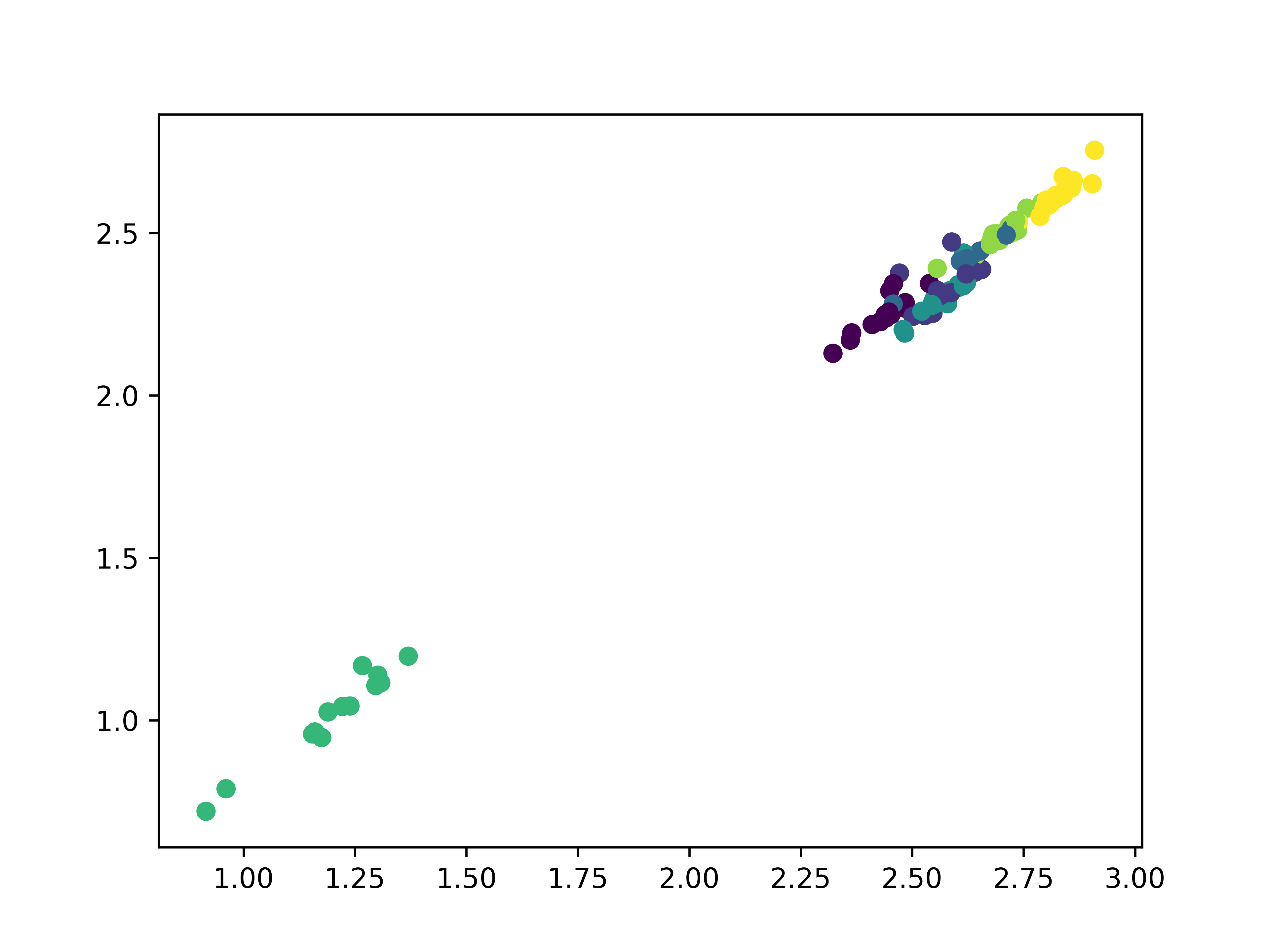
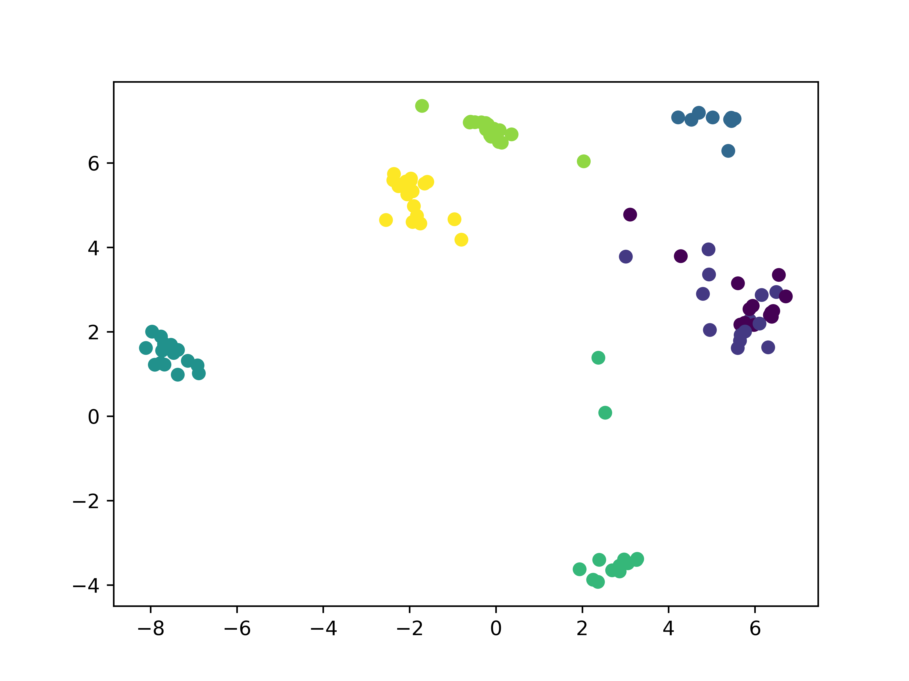
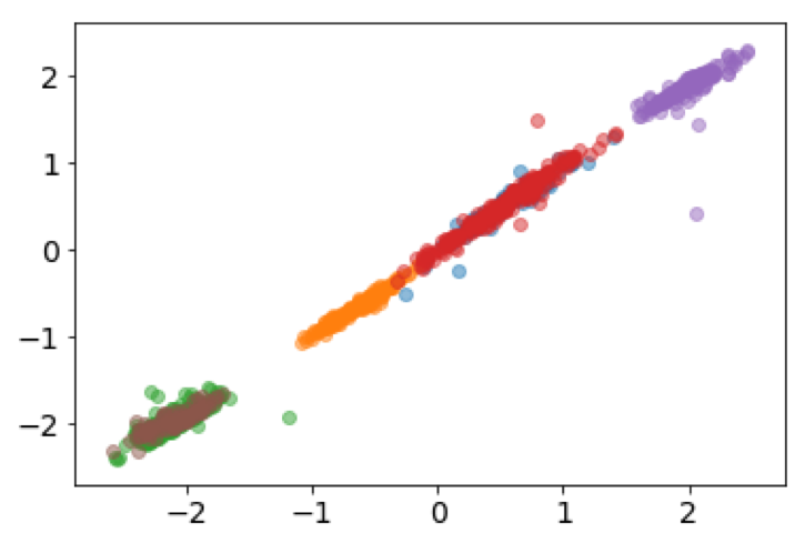
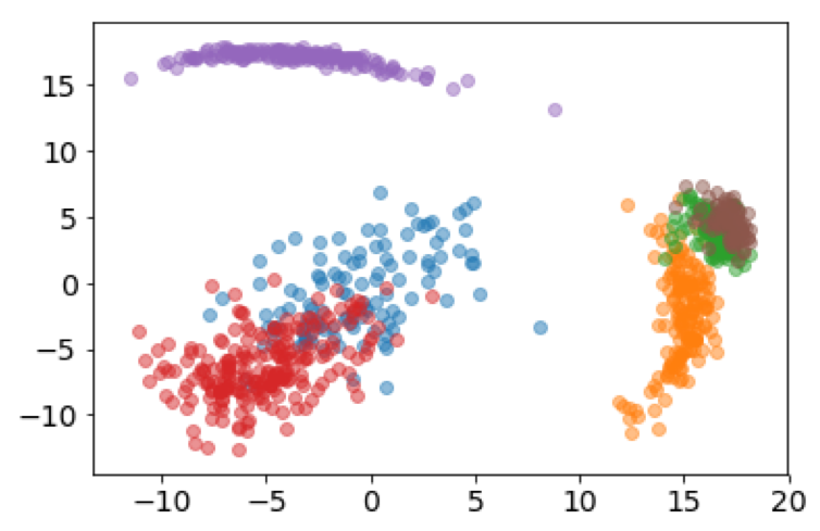
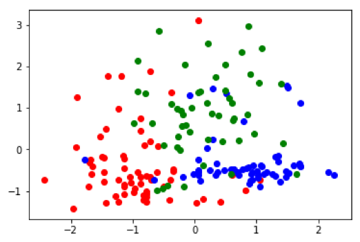
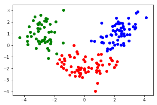
From the above plots we can see how the subspace projections help to identify components of the original dataset's feature space that produce the most separation between clusters. Additionally, with the introduction of the randomized matrix decomposition our algorithm is running much faster than the original subspace k-means algorithm.