Jacob Senecal

Computational Fluid Dynamics

2018-07-13

I worked in a computational fluid dynamics research lab during my undergrad years. In the lab we focused on developing new computational techniques to more efficiently simulate fluid dynamics phenomena. One of the main projects I worked on was to develop a new algorithm to more accurately calculate the curvature of liquid droplets in a multiphase flow. I presented the results of my work at an American Physical Society conference, and we also published our results to the Journal of Computational Physics.

An example of a multiphase flow simulation is shown above. This particular simulation is of a liquid being injected into a gas cross-flow. This kind of enviroment would be encountered in a jet engine for example.

Many gas-liquid flows are controlled by the dynamics at the phase interface, particularly the surface tension force. For example, in the atomization of a liquid fuel into droplets, the surface tension force controls the growth of interfacial instabilities that break apart the liquid core, forming ligaments and droplets that may again break apart if the flow inertia is larger than the surface tension force. For predictive simulations, of this and other gas-liquid flows, the surface tension force needs to be accurate and should converge with mesh refinement.

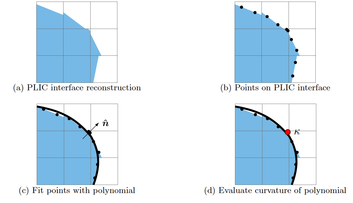
Our new algorithm computes the interface curvature by fitting a polynomial to interfacial points computed from what's known as a volume of fluid interface representation. The fit is performed with a weighted least squares regression.

To calculate the curvature of a phase interface, points are assigned to the "PLIC" which is a piecewise linear interface reconstruction. Once the points are assigned, a polynomial is fit to the points and the curvature of the polynomial is then calculated and used to represent the curvature of the interface.

The points used in the least squares method are weighted using a Gaussian distribution. What this means in practice is that points nearer to the location where the interface curvature is being calculated have a greater influence on the polynomial that is fit to the interface points, and consequently points nearer to the location where where the interface curvature is being calculated have a greater influence on the final curvature calculation itself.

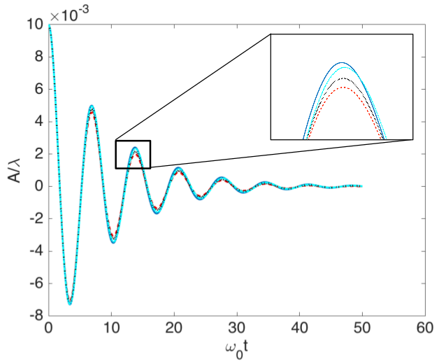
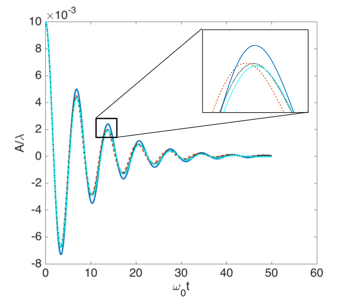
In this study the Gaussian distribution parameters were varied to change the scale the curvature is computed on (i.e. vary how much influence near and far points have on the line of best fit, and by extension the curvature calculation). The impact of the curvature scale was assessed for an oscillating droplet and a standing wave test case. These are test cases that are simple enough to have analytical solutions to use as a baseline measurement.

Standing wave test cases using a mesh of 16, 32, and 64 cells is shown by the red dashed line, black dotted line, and cyan dashed-dotted line, respectively. The analytical solution is shown by the solid blue line.

In the figures above, the image on the left shows the standing wave test case solved numerically where the polynomial fit used to calculate interface curvature was calculated using a rather narrow Gaussian distribution to weight the points that were fit to the interface. The image on the right used a Gaussian distribution that was twice as wide.

In a nutshell it turns out that it's important to balance how the points along the interace are weighted when fitting a polynomial to compute the interface curvature, with the grid resolution the curvature is being computed on. For a much more detailed analysis see our paper in the Journal of Computational Physics.